Train a Logic Classifier

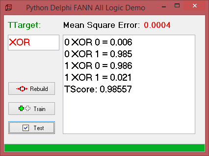
The model below this article depicts the architecture for a multilayer perceptron network designed specifically to solve the XOR problem, but all the remaining 15 logic-problems too. This I want to show with all the solutions of the FANN Library implementation in 3 steps: Build, Train and Test the NN.

A detailed report of this Classifier is available at: http://www.softwareschule.ch/download/maxbox_starter56.pdf

Fast Artificial Neural Network (FANN) Library is a free open source neural network library, which implements multilayer artificial neural networks in C , Pascal or Python with support for both fully connected and sparsely connected networks.

Once the FANN network is trained, the output unit should predict the output you would expect if you were to parse the input values through an XOR logic gate. That is, if the two input values are not equal (1,0 or 0, 1), the output should be 1, otherwise the output should be 0. As we know the XOR logic is just one of sixteen possibilities, see below.

By the way in reinforcement learning is all about making decisions sequentially. In simple words we can say that the output depends on the state of the current input and the next input depends on the output of the previous input. Ok., our all logic table for training has the following input with the most important in bold:

• All Boolean Functions
• 00000000 01 False
• 00001000 02 AND
• 00000010 03 Inhibit
• 00001010 04 Prepend
• 00000100 05 Praesect
• 00001100 06 Postpend
• 00000110 07 XOR
• 00001110 08 OR
• 11110001 09 NOR
• 11111001 10 Aequival
• 11110011 11 NegY
• 11111011 12 ImplicatY
• 11110101 13 NegX
• 11111101 14 ImplicatX
• 11110111 15 NAND
• 11111111 16 True

Before we build the NN with 3 layers here I show the implementation of the boolean logic in a procedure which is the base of the training-set, in other words, it has a positive effect on behavior:

Procedure AllBooleanPattern(aX, aY: integer);
begin
    Writeln(#13#10+'************** All Booolean Functions **************');
    PrintF('%-26s 01 False',[inttobinbyte(0)])
    PrintF('%-26s 02 AND',[inttobinbyte(aX AND aY)])
    PrintF('%-26s 03 Inhibit',[inttobinbyte(aX AND NOT aY)])
    PrintF('%-26s 04 Prepend',[inttobinbyte(aX)])
    PrintF('%-26s 05 Praesect',[inttobinbyte(NOT aX AND aY)])
    PrintF('%-26s 06 Postpend',[inttobinbyte(aY)])
    PrintF('%-26s 07 XOR',[inttobinbyte(aX XOR aY)])
    PrintF('%-26s 08 OR',[inttobinbyte(aX OR aY)])
    PrintF('%-26s 09 NOR',[inttobinbyte(NOT(aX OR aY))])
    PrintF('%-26s 10 Aequival',[inttobinbyte((NOT aX OR aY)AND(NOT aY OR aX))])
    PrintF('%-26s 11 NegY',[inttobinbyte(NOT aY)])
    PrintF('%-26s 12 ImplicatY',[inttobinbyte(aX OR NOT aY)])
    PrintF('%-26s 13 NegX',[inttobinbyte(NOT aX)])
    PrintF('%-26s 14 ImplicatX',[inttobinbyte(NOT aX OR aY)])
    PrintF('%-26s 15 NAND',[inttobinbyte(NOT(aX AND aY))])
    PrintF('%-26s 16 True',[inttobinbyte(NOT 0)])
end;

Now we want to build the NN and his architecture. This configuration should be a manual process, something based on experiences and it should be noted that the results below are for one specific model and dataset. The ideal hyper-parameters for other models and datasets will differ.:

 NN:= TFannNetwork.create(self)
  with NN do begin
    {Layers.Strings:= ('2' '3' '1') }
    Layers.add('2')
    Layers.add('3')
    Layers.add('1')
    LearningRate:= 0.699999988079071100
    ConnectionRate:= 1.000000000000000000
    TrainingAlgorithm:= taFANN_TRAIN_RPROP
    ActivationFunctionHidden:= afFANN_SIGMOID
    ActivationFunctionOutput:= afFANN_SIGMOID
    //Left := 192  //Top := 40
  end

The learning rate are the steps between and is a hyper-parameter that controls how much we are adjusting the weights of our network with respect the loss gradient as a difference or delta parameter. The lower the value, the slower we travel along the downward slope. Learning rate is applied every time the weights are updated via the learning rule; thus, if learning rate changes during training (which we don’t), the network’s evolutionary path toward its final form will immediately be altered. Connection rate of 1 means simply fully connected between neurons. Then we train the model based on our logic table with 5000 epochs:

procedure TForm1btnTrainClick(Sender: TObject);
var inputs: array [0..1] of single;
    outpts: array [0..0] of single;
    //outputs: array of single;
    e,i,j: integer;
    mse: single;
begin
    //Train the neural network epochs
   MemoXOR.Lines.Clear; 
   for e:= 1 to TRAIN_EPOCHS do begin   //Train n epochs
      epochs.Position:= e div 1;
         for i:= 0 to 1 do begin
               for j:= 0 to 1 do begin
                     inputs[0]:=i;
                     inputs[1]:=j;
                     case JStrUpper(trim(edtrule.text)) of 
                       'AND' : outpts[0]:= (i And j);
                       'NAND': outpts[0]:= 1-(i And j);
                       'OR'  : outpts[0]:= (i Or j);
                       'XOR' : outpts[0]:= (i XOr j);
                       'NOR' : outpts[0]:= 1-(i Or j);
                       'IMP' : outpts[0]:= (i Or (1-j));
                       'AEQ' : outpts[0]:= 1-(i XOr j);
                       'TAU' : outpts[0]:= 1;
                       else outpts[0]:= (i XOr j);
                     end;   
                     Mse:=NN.Train(inputs,outpts);
                     if e mod 4 = 0 then 
                        lblMse.Caption:=Format('%.4f',[Mse]);
                     Application.ProcessMessages;
               end;
         end;
      if e mod 10 = 0 then      
         MemoXor.Lines.Add(Format('%d error log = %.4f',[e, MSE]));
   end;
   ShowMessage('Network Epoch '+itoa(TRAIN_EPOCHS)+' Training Ends...');
   Writeln('Network Epoch '+itoa(TRAIN_EPOCHS)+' Training Ends...');
end;

As you can see the XOR is one of the 8 above logic functions (for sake of overview we cant see all 16 cases). The first thing we’ll explore is how learning rate affects model training. In each run the same model is trained from scratch, varying only the optimizer and learning rate. We test that with the MSE, Mse:=NN.Train(inputs,outpts);

In Statistics, Mean Square Error (MSE) is defined as Mean or Average of the square of the difference between actual and estimated values. In each run, the network is trained until it achieves at least 96% train accuracy with a low MSE.

As a target with XOR

This configuration now is not a manual process, but rather something that occurs automatically through a process known as backward propagation. Backward propagation considers the error of the prediction made by forward propagation and parses those values backwards through the network, adjusting the weights to values that slightly improve prediction accuracy.

https://www.mlopt.com/?tag=xor

Forward and backward propagation are repeated for each training example in the dataset many times until the weights of the network are tuned to values that result in forward propagation producing accurate output in the following test routine (run means test routine).

procedure TForm1btnRunClick(Sender: TObject);
var i,j, perfcnt: integer;
    perf1: single;
    inputs: array [0..1] of single;
    //output: array of fann_type;
     aoutput: TFann_Type_Array3;
begin
     MemoXOR.Lines.Clear;
     setlength(aoutput, 4)
     perf1:= 0.0; perfcnt:= 0;
     //NN.Run(inputs,aoutput);
     for i:=0 to 1 do begin
        for j:=0 to 1 do begin
           inputs[0]:=i;
           inputs[1]:=j;
           // test and predict
           NN.Run4(inputs,aoutput);
           MemoXor.Lines.Add(Format('%d '+JStrUpper(trim(edtrule.text))
                                            +' %d = %.3f',[i,j,aOutput[0]])); 
           //writeln(floattostr(nn.learningmometum))
           if aOutput[0] > PERF_GATE then begin
               perf1:= perf1 + aOutput[0];
               inc(perfcnt)
           end;     
       end;
     end;
     writeln('Test Score: '+floattostr(perf1 / perfcnt))
     MemoXor.Lines.Add(Format('TScore: %.5f',[perf1 / perfcnt]));
end;

So the score is a simple accuracy based on a threshold with a const: PERF_GATE = 0.85; Any value of 0.85 or higher is deemed to predict 1, while anything lower than 0.85 is deemed to predict 0. This is compared to the actual expected output and the proportion of correct predictions (prediction accuracy) is returned to the console. The first three parameters of the Multilayer Perceptron constructor define the dimensions of the network. In this case we have defined two input units, three hidden units and one output unit, as is required for this architecture.

Build NN with 3 layers:
NN 0: with 2
NN 1: with 3
NN 2: with 1

Also possible is to to call direct the functions via DLL for example:

Const TRAIN_EPOCHS = 5000; 
      PERF_GATE = 0.85; 
      
      function  fann_get_total_neurons: longint;
         external 'fann_get_total_neurons@fannfloat.dll stdcall';
      function  fann_print_parameters: Longint;
         external 'fann_print_parameters@fannfloat.dll stdcall';   

The script you can found at:

http://www.softwareschule.ch/examples/fanndemo.txt

As the earlier results show, it’s crucial for model training to have an good choice of optimizer and learning rate. Manually choosing these hyper-parameters is time-consuming and error-prone.

More about FANN: http://leenissen.dk/fann/wp/

Mulhouse Cité du Train

Aquitaine at Mulhouse: OLYMPUS DIGITAL CAMERA

on the left side CC 6572, OLYMPUS DIGITAL CAMERA

Base Schema for Multi-Label classification problem

initialize binary relevance multi-label

from sklearn.model_selection import train_test_split
X_train,X_test,y_train,y_test= train_test_split(X,y,test_size=0.33,random_st
classifier.fit(X_train, y_train)
BinaryRelevance(classifier=GaussianNB(), require_dense=[True, True])
predictions = classifier.predict(X_test)
accuracy_score(y_test,predictions)
0.7878787878787878

from sklearn.metrics import accuracy_score
from sklearn.model_selection import train_test_split
from sklearn.datasets import make_multilabel_classification
# using binary relevance module
from skmultilearn.problem_transform import BinaryRelevance
from sklearn.naive_bayes import GaussianNB

# this will generate a random multi-label dataset
X,y=make_multilabel_classification(sparse=True,n_labels=20,return_indicator='sparse',allow_unlabeled=False)

X<100x20 sparse matrix of type '<class 'numpy.float64'>'
        with 1812 stored elements in Compressed Sparse Row format>
y<100x5 sparse matrix of type '<class 'numpy.int32'>'
        with 477 stored elements in Compressed Sparse Row format>

# initialize binary relevance multi-label with gaussian naive bayes base classifier
classifier = BinaryRelevance(GaussianNB())

X_train,X_test,y_train,y_test= train_test_split(X,y,test_size=0.33, random_state=42)

classifier.fit(X_train, y_train)
BinaryRelevance(classifier=GaussianNB(),require_dense=[True,True])

predictions = classifier.predict(X_test)
accuracy_score(y_test,predictions)
>>>0.7878787878787878
>>>

# another approach with powerset instead of subset
# transforms this problem into a single multi-class problem 

from skmultilearn.problem_transform import LabelPowerset
classifier = LabelPowerset(GaussianNB())
classifier.fit(X_train, y_train)
LabelPowerset(classifier=GaussianNB(),require_dense=[True,True])
predictions = classifier.predict(X_test)
accuracy_score(y_test,predictions)
>>>0.8484848484848485
>>>

Python Bus

Solving Multi-Label Classification problems (Case studies included)

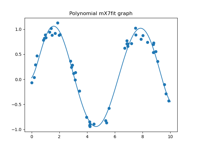
Base Schema for Polynomial Regression

What is a straightforward way of doing multivariate polynomial regression for python?

import numpy as np
import matplotlib.pyplot as plt
from sklearn.preprocessing import PolynomialFeatures
from sklearn.linear_model import LinearRegression
from sklearn.pipeline import make_pipeline

rng=np.random.RandomState(1)
# get some sin data
X=10 * rng.rand(50)
y=np.sin(X)+0.1*rng.randn(50)

poly=make_pipeline(PolynomialFeatures(degree=7),LinearRegression())
Xfit=np.linspace(0,10,1000)
# train and predict
poly.fit(X[:,np.newaxis],y)
>>>Pipeline(steps=[('polynomialfeatures', PolynomialFeatures(degree=7)),
                ('linearregression', LinearRegression())])
yfit=poly.predict(Xfit[:,np.newaxis])
# plot it
plt.scatter(X,y)
>>><matplotlib.collections.PathCollection object at 0x000000523600E470>
plt.title("Polynomial mX7fit graph")
>>>Text(0.5, 1.0, 'Polynomial mX7fit graph')
plt.plot(Xfit, yfit)
>>>[<matplotlib.lines.Line2D object at 0x0000005236C1CF28>]
plt.show()

coefficients = poly.steps[1][1].coef_
intercepts = poly.steps[1][1].intercept_
coefficients.shape
(8,)

coefficients
array([ 0.00000000e+00, 3.31250195e-01, 1.28845777e+00, -1.06474496e+00,
2.90659230e-01, -3.57011703e-02, 2.01614684e-03, -4.20513336e-05])

For every response variable, it appears we end up with 8 coefficients + one intercept (in our case not), which is one more coefficient than I would expect. We have 50 sample points to fit.

ML Primer

Our first goal is to predict a credit situation called creditworthy, so we want to know if a person can pay back a debt;

This is a supervised classifier as a binary classifier called logistic regression:

Log Regression first

import numpy as np
from matplotlib import pyplot as plt
from sklearn.linear_model import LogisticRegression
X=np.array([[10000,80000,35],[7000,120000,57],[100,23000,22],[223,18000,26]])
y=np.array([1,1,0,0])

cls=LogisticRegression(random_state=12)
cls.fit(X,y)
LogisticRegression(random_state=12)
print(cls.predict([[6500,50000,26]]))
>>> [1]
>>>

So this is at one point the equation to solve: a + bx = y , e.g. 10 + 20x = 50

coefficients with intercept

Each service of a cloud-native machine learning application is developed using the language and framework best suited for the functionality. Cloud-native applications are polyglot. Services use a variety of languages, run-times and frameworks. For example, developers may build a real-time streaming service based on Web Sockets, developed in Node.js, while choosing Python for building a machine learning based service and choosing spring-boot for exposing the REST APIs. The fine-grained approach to developing micro-services lets them choose the best language and framework for a specific job.

important terms

Trade off between false positive or false negative

Precision oriented wants to reduce false positives, for example a doctor says no one has a disease, but false negatives grow. False positive refers to a test result that tells you a disease or condition is present, when in reality, there is no disease. A false positive result is an error, which means the result is not giving you the correct information. As an example of a false positive, suppose a blood test is designed to detect colon cancer. The test results come back saying a person has colon cancer when he actually does not have this disease. This is a false positive.

A false negative error, or false negative, is a test result which wrongly indicates that a condition does not hold. For example, when a pregnancy test indicates a woman is not pregnant, but she is, or when a person guilty of a crime is acquitted, these are false negatives. The condition “the woman is pregnant”, or “the person is guilty” holds, but the test (the pregnancy test or the trial in a court of law) fails to realize this condition, and wrongly decides that the person is not pregnant or not guilty.

https://en.wikipedia.org/wiki/False_positives_and_false_negatives

Trade off as The “power” (or the “sensitivity“) of the test is equal to 1 − β.

The Null hypothesis states no disease and Alt states a person has a disease. If the decision boundary goes to the right a doctor has an attendance to say you don’t have the disease so he wants to minimize alpha as false positive!

He wants to make sure only strong symptoms shows the disease but on the other side people with weak symptoms fail the test and don’t realize that they have the disease (false negative as beta grows).

CAS PML April 2021

Teams versus Zoom versus Skype

TeamsZoomSkype

Maurienne Strasbourg

OLYMPUS DIGITAL CAMERA

OLYMPUS DIGITAL CAMERA

L.S. Models CC